Analyzing Stability Properties

Plotting the region of absolute stability

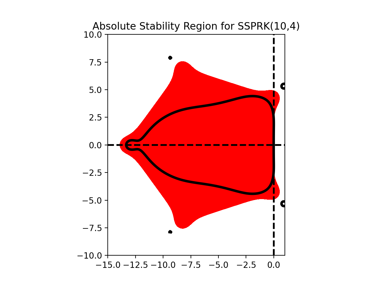
Region of absolute stability for the optimal SSP 10-stage, 4th order Runge-Kutta method:

from nodepy.runge_kutta_method import *
ssp104=loadRKM('SSP104')
ssp104.plot_stability_region(bounds=[-15,1,-10,10])

(Source code, png, hires.png, pdf)

RungeKuttaMethod.plot_stability_region(N=200, color='r', filled=True, bounds=None, plotroots=False, alpha=1.0, scalefac=1.0, to_file=False, longtitle=True, fignum=None)

The region of absolute stability of a Runge-Kutta method, is the set

$$ \{ z \in C : | \phi(z) | \le 1 \} $$

where \(\phi(z)\) is the stability function of the method.

Input: (all optional)

• N – Number of gridpoints to use in each direction

• bounds – limits of plotting region

• color – color to use for this plot

• filled – if true, stability region is filled in (solid); otherwise it is outlined

Example::

>>> from nodepy import rk
>>> rk4 = rk.loadRKM('RK44')
>>> rk4.plot_stability_region() 
<Figure size...

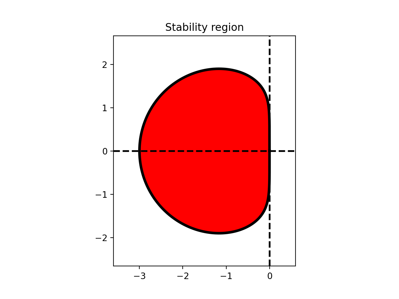
Region of absolute stability for the 3-step Adams-Moulton method:

from nodepy.linear_multistep_method import *
am3=Adams_Moulton(3)
am3.plot_stability_region()

(Source code, png, hires.png, pdf)

LinearMultistepMethod.plot_stability_region(N=100, bounds=None, color='r', filled=True, alpha=1.0, to_file=False, longtitle=False)

The region of absolute stability of a linear multistep method is the set

$$ \{ z \in C \mid \rho(\zeta) - z \sigma(\zeta) \text{ satisfies the root condition} \} $$

where \(\rho(\zeta)\) and \(\sigma(\zeta)\) are the characteristic functions of the method.

Also plots the boundary locus, which is given by the set of points z:

$$ \{z \mid z = \rho(\exp(\imath \theta)) / \sigma(\exp(\imath\theta)), 0 \le \theta \le 2\pi \} $$

Here \(\rho\) and \(\sigma\) are the characteristic polynomials of the method.

Reference: [LeV07] section 7.6.1

Input: (all optional)

• N – Number of gridpoints to use in each direction

• bounds – limits of plotting region

• color – color to use for this plot

• filled – if true, stability region is filled in (solid); otherwise it is outlined

Plotting the order star

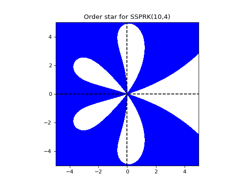
Order star for the optimal SSP 10-stage, 4th order Runge-Kutta method:

from nodepy.runge_kutta_method import *
ssp104=loadRKM('SSP104')
ssp104.plot_order_star()

(Source code, png, hires.png, pdf)

RungeKuttaMethod.plot_stability_region(N=200, color='r', filled=True, bounds=None, plotroots=False, alpha=1.0, scalefac=1.0, to_file=False, longtitle=True, fignum=None)

The region of absolute stability of a Runge-Kutta method, is the set

$$ \{ z \in C : | \phi(z) | \le 1 \} $$

where \(\phi(z)\) is the stability function of the method.

Input: (all optional)

• N – Number of gridpoints to use in each direction

• bounds – limits of plotting region

• color – color to use for this plot

• filled – if true, stability region is filled in (solid); otherwise it is outlined

Example::

>>> from nodepy import rk
>>> rk4 = rk.loadRKM('RK44')
>>> rk4.plot_stability_region() 
<Figure size...